
What is Hypothesis Testing
Hypothesis Testing allows Six Sigma team to draw conclusions about the population based on statistical analysis performed on a sample. Because the conclusions are based on samples and not the entire population, there is always some risk of error.
Using the information about the sample, statistically the p-value of the data collected can be calculated. p-value is the mean to tell if the assumption or conclusion drawn on the sample is correct or not.
Normal Probability Distribution
Normal Distribution, also called Gaussian distribution, is probably the most important distribution related to continuous data from statistical analysis standpoint.
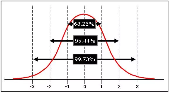
Since many natural process outcomes are normally distributed, Six Sigma relies on this curve and the Empirical Rule (68-95-99.7%) to assess how well a process meets specifications and whether a sample size is good enough to be used for analysis.
In a perfect normal distribution, 68.26% of all data points fall within plus or minus 1 standard deviation from the mean; 95.46% of the data points fall within plus or minus 2 standard deviation from the mean; and 99.73% of the data points fall within plus or minus 3 standard deviation from the mean.
Testing whether data is normal is critical in statistical analysis because the results of tests conducted can be invalid if the accuracy of the data is not accounted for.
To determine if the sample data used is normal, advanced statistics are required. Microsoft Excel and other programs can be used to perform the calculation before the data is to conduct required analysis.
How to use Excel to check if sample data is normal
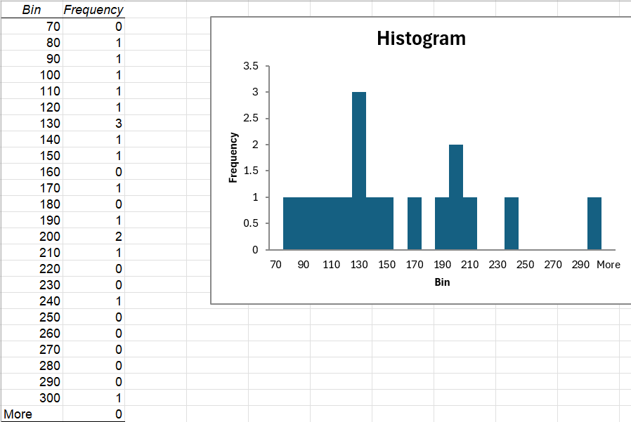
1. Create a Histogram using the sample data. Using the example of Time taken for Adults to complete the 100m Swim, the following Histogram is created.
2. The Descriptive Statistical information of the data set is created as followed
| Mean | 155.4117647 |
| Standard Error | 14.14578996 |
| Median | 134 |
| Mode | #N/A |
| Standard Deviation | 58.32458618 |
| Sample Variance | 3401.757353 |
| Kurtosis | 0.815962627 |
| Skewness | 0.990489892 |
| Range | 220 |
| Minimum | 80 |
| Maximum | 300 |
| Sum | 2642 |
| Count | 17 |
3. The Expected Distribution and the Observed Distribution are calculated as followed
| Bin Range | CDF to left | Bin Only | Expected Number | Observed | (Exp – Obs)2 | Divided by Exp |
| 70 | 0.07153944 | 0.07153944 | 1.216170474 | 0 | 1.47907062 | 1.216170474 |
| 80 | 0.098011238 | 0.026471798 | 0.45002057 | 1 | 0.30247737 | 0.672141216 |
| 90 | 0.131034842 | 0.033023604 | 0.561401273 | 1 | 0.19236884 | 0.342658366 |
| 100 | 0.171041282 | 0.04000644 | 0.680109482 | 1 | 0.10232994 | 0.150460986 |
| 110 | 0.218106468 | 0.047065185 | 0.800108148 | 1 | 0.03995675 | 0.049939189 |
| 120 | 0.27187573 | 0.053769262 | 0.914077456 | 1 | 0.00738268 | 0.00807665 |
| 130 | 0.331528805 | 0.059653075 | 1.014102274 | 3 | 3.94378978 | 3.888946783 |
| 140 | 0.395796993 | 0.064268188 | 1.0925592 | 1 | 0.00856721 | 0.007841411 |
| 150 | 0.46303638 | 0.067239388 | 1.143069588 | 1 | 0.02046891 | 0.017906965 |
| 160 | 0.531351356 | 0.068314975 | 1.161354579 | 0 | 1.34874446 | 1.161354579 |
| 170 | 0.59875332 | 0.067401965 | 1.145833402 | 1 | 0.02126738 | 0.018560622 |
| 180 | 0.663332671 | 0.064579351 | 1.097848959 | 0 | 1.20527234 | 1.097848959 |
| 190 | 0.723419496 | 0.060086825 | 1.021476033 | 1 | 0.00046122 | 0.000451523 |
| 200 | 0.77771068 | 0.054291184 | 0.922950123 | 2 | 1.16003644 | 1.256878794 |
| 210 | 0.825347616 | 0.047636936 | 0.809827904 | 1 | 0.03616543 | 0.044658162 |
| 220 | 0.865937963 | 0.040590347 | 0.690035899 | 0 | 0.47614954 | 0.690035899 |
| 230 | 0.89952457 | 0.033586608 | 0.570972328 | 0 | 0.3260094 | 0.570972328 |
| 240 | 0.926512771 | 0.0269882 | 0.458799406 | 1 | 0.29289808 | 0.63840118 |
| 250 | 0.947572176 | 0.021059405 | 0.35800989 | 0 | 0.12817108 | 0.35800989 |
| 260 | 0.96353033 | 0.015958154 | 0.271288615 | 0 | 0.07359751 | 0.271288615 |
| 270 | 0.975273451 | 0.011743121 | 0.199633057 | 0 | 0.03985336 | 0.199633057 |
| 280 | 0.983665127 | 0.008391677 | 0.142658502 | 0 | 0.02035145 | 0.142658502 |
| 290 | 0.989488549 | 0.005823421 | 0.098998165 | 0 | 0.00980064 | 0.098998165 |
| 300 | 0.993412937 | 0.003924388 | 0.066714599 | 1 | 0.87102164 | 13.05593757 |
4. Using the result above, the p-Value can be calculated using the Chi-Squared formula in Excel, and it is derived as 0.207984876. And it is good since the p-Value is greater than 0.05
| Total x2 | 25.95982989 |
| Degree of Freedom | 21 |
| CHISQ.DIST | 0.207984876 |